In this article we will cover the problems of overfitting and under-fitting during the training of your Neural Network and the potential remedies you can employ to avoid it. It will enable you to train networks which will generalize well over previously unseen test samples.
What is Overfitting and Underfitting?
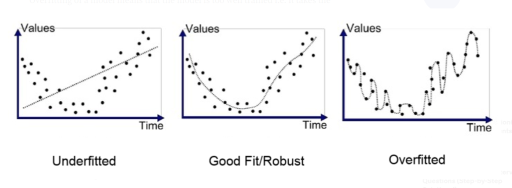
When the Neural network fits the training data so perfectly that it does not generalizes well on the test data, we say that the network has overfitted the training data. We can spot this during training – if the training accuracy is more than validation set accuracy, it signals Overfitting.
Under-fitting is when the model has too few parameters that it has lower accuracy on training set itself, where it leaves too much on the table and fails to extract relevant patterns from the training data.
Below are some graphs showing, under-fit, good-fit and over-fit models respectively.
How to identify if your network is over-fitting?
If the training set accuracy is more than the validation set accuracy, it signals overfitting in the network
How to identify if your network is under-fitting?
If the error rate on training set is high, it signals under-fitting
How to avoid under-fitting and over-fitting?
It is a tradeoff between how well you want to fit the training dataset and also keep a good accuracy on the validation and test set by preventing over-fitting.
Main goal is to keep generalization error (accuracy on test set) to be low by having just enough parameters that validation accuracy always stays more than training accuracy and test error rate is minimum.
Below mentioned techniques help in minimizing the problems of over and under fitting in Neural network training
Regularization
Regularization is the constraint which keeps both the sides in balance. Tuning the regularization parameter to such an extent that the model has just the right degree of freedom so that it generalizes well outside of the training dataset.
There are various techniques that you can employ to implement regularization for your Neural Network. Below, we will look at all these techniques and also the ways to implement them in Keras
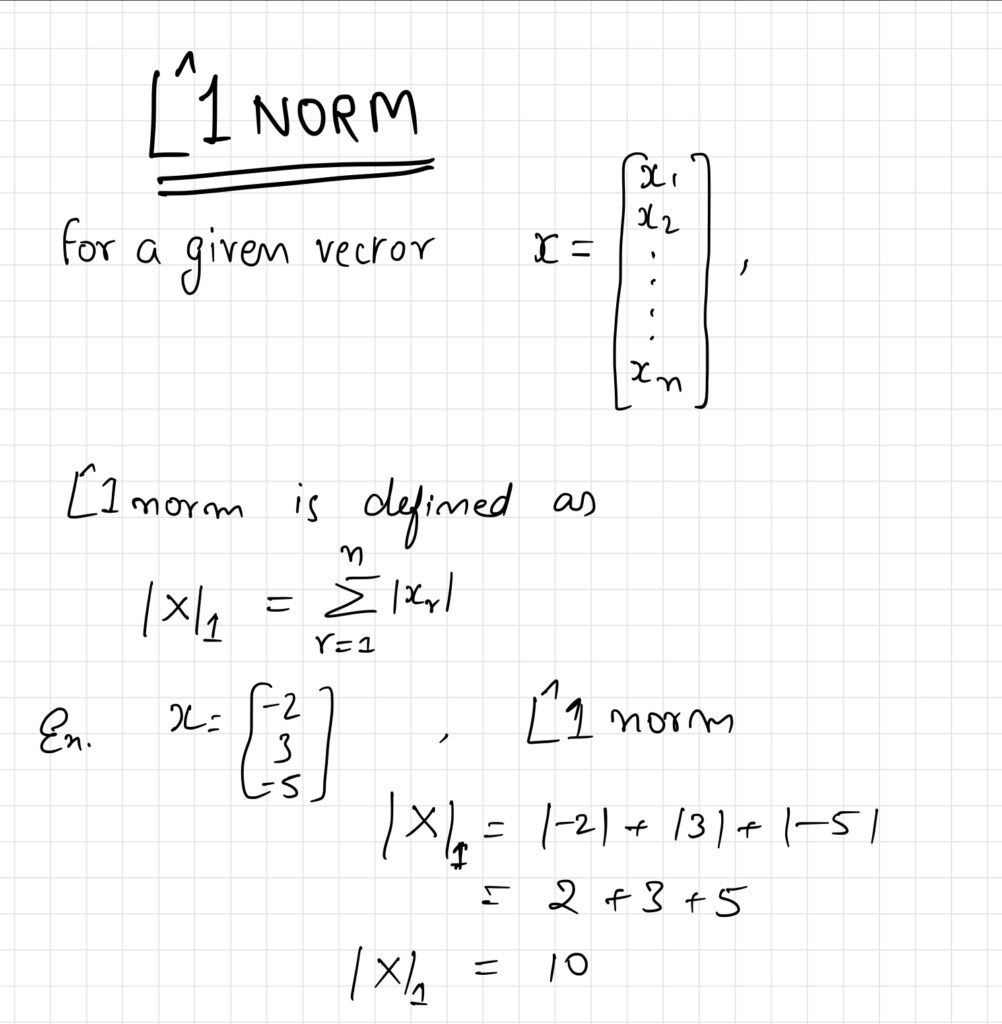
1. L1 and L2 Regularization
L1 regularization makes use of the L1 norm and drives some of the weights of the network to zero essentially resulting in a sparse model.
L1 Keras Implementation
You will need to apply these regularizer to all the layers in your network.
layer = tf.keras.layers.Dense(100, activation="relu",
                              kernel_initializer="he_normal",
                              kernel_regularizer=tf.keras.regularizers.l1(0.01))
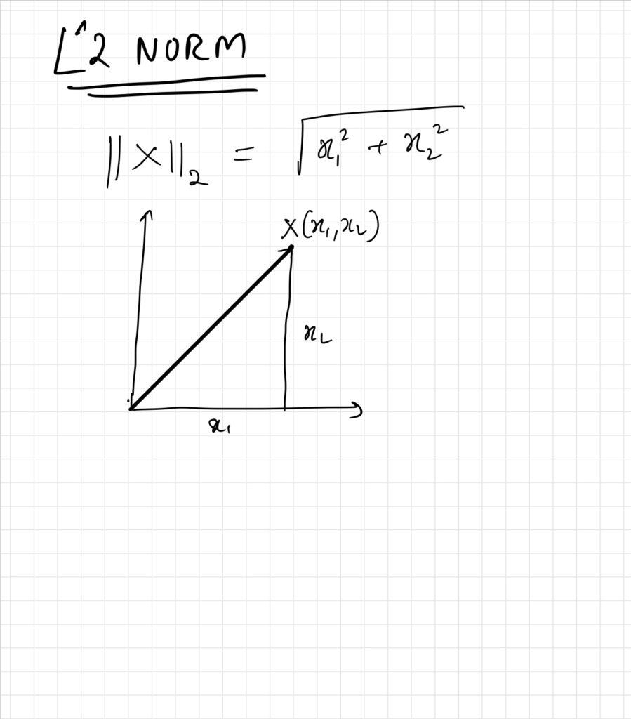
L2 regularization makes use of the L2 norm and constrains the weights of the neural network from taking too large values.
L2 Keras Implementation
You will need to apply these regularizer to all the layers in your network.
layer = tf.keras.layers.Dense(100, activation="relu",
                              kernel_initializer="he_normal",
                              kernel_regularizer=tf.keras.regularizers.l2(0.01))
L1 and L2 methods return a regularizer that will be called at each step during the training to compute the regularization loss, which is then added to the final loss.
Regularization Factor
You can think of it as the strength of regularization as to how much penalty will be applied to the weights. Higher the value more the weights will be drawn to zero (in case of l1) or will be restricted in a range (in case of l2).
How to apply both L1 and L2 Regularization in Keras?
You will need to apply these regularizer to all the layers in your network.
layer = tf.keras.layers.Dense(100, activation="relu",
                              kernel_initializer="he_normal",
                              kernel_regularizer=tf.keras.regularizers.l1_l2(l1=0.1,l2=0.01))
2. Batch Normalization
Batch Normalization layer, which is used to overcome vanishing and exploding gradients, also acts as a really good regularizer. You can read more about this technique in detail in my earlier article on vanishing and exploding gradients here
3. Dropout
Dropout is one of the most successful regularization technique used by many state of the art neural network architectures. It was proposed in a paper26 by Geoffrey Hinton et al. in 2012 and further detailed in a 2014 paper27 by Nitish Srivastava et al.
In this technique, during training, some of the neurons are turned off and do not participate in the training during that epoch, effectively resulting in a new new neural network at each step. This generates an ensemble of multiple neural networks.
At each training step every neuron including the input neurons, but always excluding the output neurons), has a probability p of being temporarily “dropped out” of that training step, but it may be active in the next step.
Dropout Rate
Hyper-parameter p, called the dropout rate controls the probability of a neuron being turned off during that training step.
It is typically set between 10% and 50%, between 20%-30% for recurrent neural networks and between 40%-50% for convolutional neural nets.
At each training step since each neuron can be either present or absent, therefore effectively it generates a total of 2^N possible unique networks.
Once you have run 10,000 training steps, you have essentially trained 10,000 different neural networks. The resulting neural network can be seen as an averaging ensemble of all these smaller neural networks.
After the training neurons don’t get dropped anymore
Important Technical Detail about Dropout
Suppose Dropout Rate is set to p=75%, that means on average only 25% of the all neurons will be active at each training step.
It results in each neuron being connected to 4 times as many input neurons. As we know after training the neurons will not dropout anymore, therefore the neural network will see different data during and after training.
To compensate for this we need to divide the connection weights by the Keep Probability (1 – p) during training. Keras automatically does this for you.
Implementing Dropout in Keras
model = tf.keras.Sequential([
    tf.keras.layers.Flatten(input_shape=[28, 28]),
    tf.keras.layers.Dropout(rate=0.2),
    tf.keras.layers.Dense(100, activation="relu",
                          kernel_initializer="he_normal"),
    tf.keras.layers.Dropout(rate=0.2),
    tf.keras.layers.Dense(100, activation="relu",
                          kernel_initializer="he_normal"),
    tf.keras.layers.Dropout(rate=0.2),
    tf.keras.layers.Dense(10, activation="softmax")
])
In the above code a dropout (of 20%) is applied to each dense layer starting from the input layer but excluding the output layer.
Tuning
If you see that the model is overfitting then increase the dropout rate or decrease it if it is under-fitting.
Another technique is to increase the dropout rate for large layers and reduce it for small ones
Many state of the art architectures only use dropout after the last hidden layer, you can try this if full dropout is too strong.
Warning
Since dropout is only active during training, comparing the training loss and validation loss can be misleading. Therefore make sure to evaluate the training loss without dropout (eg after training).
Also Dropout can significantly increase the convergence time, but it is worth the extra effort as it reduces the error rate considerably and avoids over and under-fitting.
4. Monte Carlo (MC) Dropout
Authors of the 2016 paper (Yarin Gal and Zoubin Ghahramani) on MC Dropout, established a solid mathematical connection between Dropout networks and approximate Bayesian inference.
They also proved that MC Dropout can boost the performance of any already trained dropout model without having to retrain it and that too in just a few lines of code.
Additionally, predictions using MC Dropout provided a much better measure of the model’s uncertainty.
Implementation
import numpy as np

y_probas = np.stack([model(X_test, training=True) for sample in range(100)])
y_proba = y_probas.mean(axis=0)
In the above code, model(X) is similar to model.predict() except it returns a tensor rather than a Numpy Array and it also supports a training argument.
Setting training = True ensures that dropout layer remains active so all predictions will be a bit different. In this example we are making 100 predictions over the test set and then we compare their average.
Thats all!!, averaging over multiple predictions with dropout turned on gives us Monte Carlo estimate, which is generally more reliable than a single prediction with dropout turned off.
Some example predictions are below comparing with dropout turned off vs MC Dropout (i.e. dropout turned on) on the Fashion MNIST dataset.
# with dropout turned off
>>> model.predict(X_test[:1]).round(3)
array([[0.   , 0.   , 0.   , 0.   , 0.   , 0.024, 0.   , 0.132, 0.   ,
        0.844]], dtype=float32)
# with dropout turned on - MC Dropout predictions
>>> y_proba[0].round(3)
array([0.   , 0.   , 0.   , 0.   , 0.   , 0.067, 0.   , 0.209, 0.001,
       0.723], dtype=float32)
As you can see the model predictions with dropout turned off is fairy confident at 84.4% that the item is a class 9 (i.e. ankle boot) whereas the model prediction with MC dropout is less confident at 72.3% that it is an ankle boot but the estimated probabilities of class 5 (sandal) and class 7 (sneaker) have increased, which makes sense as they are also footwear.
MC dropout tends to improve the reliability of the model’s probability estimates which means it is less likely to be confident but wrong. If a model is confidently wrong it can be very dangerous in some situations such has self driving car confidently gets the stop sign wrong and zooms past it.
MC dropout introduces caution to the predictions and also provides standard deviations of the probability estimates which are helpful in judging the uncertainty of the model. It’s also useful to know exactly which other classes are most likely
>>> y_std = y_probas.std(axis=0)
>>> y_std[0].round(3)
array([0.   , 0.   , 0.   , 0.001, 0.   , 0.096, 0.   , 0.162, 0.001,
       0.183], dtype=float32)
As you can see above there is a lot of variance in probability estimates of class 9 (0.183) which should be compared to the estimated probability of 0.72. If you are building a risk sensitive system (e.g medical or financial system), you would treat such an uncertain prediction with extreme caution.
Hyperparameter
The number of samples you use (100 in this case) is a hyper-parameter you can tune. The higher it is, the more accurate the predictions and their uncertainty estimates. However if you double it the inference time will also be doubled. Your job is to find right trade-off between latency and accuracy depending on your application
Using MC Dropout with Batch Normalization layers
If your network contains other layers which behave differently during training and predictions then you should not force training mode to True as we just did. Instead you should replace the Dropout layers with following MCDropout class
class MCDropout(tf.keras.layers.Dropout):
    def call(self, inputs, training=False):
        return super().call(inputs, training=True)
In the above code we are just subclassing the Dropout layer and override the call() method to force its training argument to True.
If you are creating a model from scratch then it is just a matter of using the MCDropout class rather than using Dropout, but if you have an already trained model using Dropout, you need to create a new model identical to existing model except with MCDropout instead of Dropout, then copy the existing model’s weights to your new model.
5. Max-Norm Regularization
For each neuron, Max-Norm regularization constrains the weights w of the incoming connections such that L2_norm(W) <= r, where r is the max-norm hyper- parameter.
Max-Norm does not add regularization loss to the overall loss functions but instead it is implemented by computing L2_Norm of W after each training step and rescaling W if needed.
Reducing r increases the amount of regularization and helps reduce overfitting. It can also alleviate the unstable gradient problem (if you are not using Batch Normalization)
Implementation in Keras
dense = tf.keras.layers.Dense(
    100, activation="relu", kernel_initializer="he_normal",
    kernel_constraint=tf.keras.constraints.max_norm(1.))
As shown above you need to set kernel_constraint argument of each hidden layer to max_norm() constraint with approximate max value. Here r is set to 1.
After each training iteration, the model’s fit() method will call the object returned by max_norm(), passing it the layer’s weights and gets rescaled weights in return.
Also you can defined your own custom constraint function and use it as the kernel_constraint. You can also constraint the bias term by setting the bias_constraint argument.
There is also an axis argument which might need tweaking of you are using it in convolutional neural networks.
Conclusion
In this article we covered various techniques to overcome the problems of over and under-fitting in neural network training. As we can see it is a balancing act between different capabilities of the network. You need to carefully plan the training and optimization of your network.
Using these techniques you can ensure that you get the maximum value out of your network training time and extract as much valuable information from the training dataset. It will ensure your network does not overfit the training data and generalizes will over previously unseen examples.
Do let me know any questions you have in the comments below.